Algorithmic concepts

By Afshine Amidi and Shervine Amidi

Overview

Algorithm

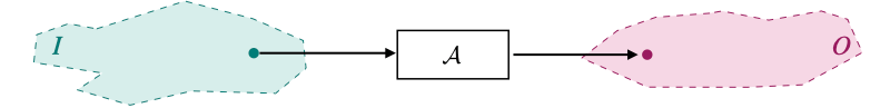
Given a problem, an algorithm $\mathcal{A}$ is a set of well-defined instructions that runs in a finite amount of time and space. It receives an input $I$ and returns an output $O$ that satisfies the constraints of the problem.

As an example, a problem can be to check whether a number is even. In order to do that, an algorithm could be to check whether the number is divisible by 2.

Iteration

An iterative algorithm is an algorithm that runs through a sequence of actions. It is characterized by either a for or a while loop.

Suppose we want to return the sum of all of the elements of a given list. An example of an iterative algorithm would be to sequentially add each element of the list to a variable, and return its final value.

Recursion

A recursive algorithm uses a function that calls itself. It is composed of the following components:

• Base case: This is the set of inputs for which the outputs are known.
• Recursive formula: The answer of the current step is based on function calls relying on previous steps, eventually using the base case answer.

A classic problem is to compute the power of a number $x^n$ without explicitly using the power operation. In order to do that, a recursive solution could rely on the following cases:

$$\begin{cases} \: x^0=1&\textrm{ is known}\\ \: x^n=x^{\frac{n}{2}}\times x^{\frac{n}{2}}&\textrm{when }n\in\mathbb{N}^*\textrm{ is even}\\ \: x^n=x\times x^{\frac{n-1}{2}}\times x^{\frac{n-1}{2}}&\textrm{when }n\in\mathbb{N}^*\textrm{ is odd} \end{cases}$$

Call stack

In a recursive algorithm, the space used by function calls $c_i$ is called the stack space.

Stack overflow

The problem of stack overflow occurs when a recursive algorithm uses more stack space than the maximum allowed $N$.

A solution to circumvent this bottleneck is to convert the code from being recursive to being iterative so that it relies on memory space, which is typically bigger than stack space.

Memoization

Memoization is an optimization technique aimed at speeding up the runtime by storing results of expensive function calls and returning the cache when the same result is needed.

Types of algorithms

Brute-force

A brute-force approach aims at listing all the possible output candidates of a problem and checking whether any of them satisfies the constraints. It is generally the least efficient way of solving a problem.

To illustrate this technique, let's consider the following problem: given a sorted array $A$, we want to return all pairs of elements that sum up to a given number.

• A brute-force approach would try all possible pairs $(a_i, a_j)$ and return those that sum up to that number. This method produces the desired result but not in minimal time.
• A non-brute-force approach could use the fact that the array is sorted and scan the array using the two-pointer technique.

Backtracking

A backtracking algorithm recursively generates potential solutions and prunes those that do not satisfy the problem constraints. It can be seen as a version of brute-force that discards invalid candidates as soon as possible.

As an example, the $N$-Queens problem aims at finding a configuration of $N$ queens on a $N\times N$ chessboard where no two queens attack each other. A backtracking approach would consist of placing queens one at a time and prune solution branches that involve queens attacking each other.

Greedy

A greedy algorithm makes choices that are seen as optimal at every given step. However, it is important to note that the resulting solution may not be optimal globally. This technique often leads to relatively low-complexity algorithms that work reasonably well within the constraints of the problem.

To illustrate this concept, let's consider the problem of finding the longest path from a given starting point in a weighted graph. A greedy approach constructs the final path by iteratively selecting the next edge that has the highest weight. The resulting solution may miss a longer path that has large edge weights "hidden" behind a low-weighted edge.

Divide and conquer

A divide and conquer (D&C) algorithm computes the final result of a problem by recursively dividing it into independent subproblems:

• Divide: The problem is divided into several independent subproblems.

  

• Conquer: Each subproblem is solved independently.

  

• Combine: The result of each subproblem is combined to find the final answer.

  

Algorithms following the D&C principle include sorting algorithms such as merge sort and quick sort.

Dynamic Programming

Dynamic programming (DP) is a method of problem resolution that relies on finding answers to overlapping subproblems.

A common example of problem resolution using DP is the computation of Fibonacci numbers.

There are two main approaches:

Top-down This approach finds the target value by recursively computing previous values.

• Step 1: Try computing the desired value $F_n$ and notice that it is based on previous values.

  

• Step 2: Try computing the previous values, which themselves rely on earlier values, some of which may have already been computed. In this case, we can use memoization to avoid duplicate operations.

  

• Step 3: Use the newly computed values to deduce $F_n$.

  

Bottom-up This approach starts from already-known results and iteratively computes succeeding values until it reaches the target value.

• Step 1: Compute $F_0$, $F_1$, $F_2$, etc. in a predetermined way. These values are typically stored in an array.

  

• Step 2: Deduce $F_n$.

  

In summary, the two main ways of solving a problem with DP are:

Top-down	Bottom-up
Recursive approach	Iterative approach

Remark

A key difference between DP and D&C strategies is that DP relies on overlapping subproblems whereas D&C bases itself on independent subproblems.

Complexity

Definition

The concept of complexity is used to quantify the efficiency of an algorithm. There are two types of complexities:

• Time: How many operations are made?
• Space: How much extra space is needed?

Both measures are usually given as a function of the input size $n$, although other parameters can also be used.

Notations

The complexity $f$ of an algorithm can be described using a known function $g$ with the notations described in the table below:

Notation	Definition	Meaning	Illustration
$f=o(g)$ "little oh of $g$"	$\forall\epsilon>0, \exists n_0, \forall n \geqslant n_0$ $\vert f(n)\vert\leqslant\epsilon\vert g(n)\vert$	Negligible compared to $g$ $f(n) \underset{n\rightarrow+\infty}{\ll} g(n)$
$f=\mathcal{O}(g)$ "big oh of $g$"	$\exists c>0, \exists n_0, \forall n\geqslant n_0$ $\vert f(n)\vert \leqslant c\vert g(n)\vert$	Upper-bounded by $g$ $f(n)\underset{n\rightarrow+\infty}{\leqslant}g(n)$
$f=\Omega(g)$ "omega of $g$"	$\exists c>0, \exists n_0, \forall n\geqslant n_0$ $\vert f(n)\vert \geqslant c\vert g(n)\vert$	Lower-bounded by $g$ $f(n)\underset{n\rightarrow+\infty}{\geqslant}g(n)$
$f=\Theta(g)$ "theta of $g$"	$\exists c_1, c_2>0, \exists n_0, \forall n\geqslant n_0$ $\vert f(n)\vert \geqslant c_1\vert g(n)\vert$ $\vert f(n)\vert \leqslant c_2\vert g(n)\vert$	Similar to $g$ $f(n)\underset{n\rightarrow+\infty}{\sim}g(n)$

Remark

The big oh notation is frequently used to describe the time and space complexity of a given algorithm.

Orders of magnitude

The table below highlights the main kinds of runtime complexities $T(n)$ as a function of the input size $n$:

Complexity	Example of application
O(1) "constant"	Hash table lookup: Accessing the value of a given key does not depend on the size of the hash table.
O(log(n)) "logarithmic"	Binary search: The search space is divided by 2 at each iteration.
O(n) "linear"	Linear search: All elements of the input are visited.
O(n log(n)) "linearithmic"	Merge sort: The array is broken down by two at every step and each step requires all elements to be checked.
O(n**2) "quadratic"	Bubble sort: Each pair of elements of the input array is checked.
O(2**n) "exponential"	0/1 knapsack problem: The naive approach would consist of trying out every combination of items in the final set.
O(n!) "factorial"	Traveling salesman problem: The naive approach consists of trying all possible permutations of cities to visit.

The following graph shows the difference in their evolutions:

As a rule of thumb, we have:

$$\boxed{\mathcal{O}(1) < \mathcal{O}(\log(n)) < \mathcal{O}(n) < \mathcal{O}(n\log(n)) < \mathcal{O}(n^2) < \mathcal{O}(2^n) < \mathcal{O}(n!)}$$

Master theorem

The master theorem gives an explicit solution of a runtime $T(n)$ that satisfies a recursive relationship of the form below:

$$\boxed{T(n)=aT\left(\frac{n}{b}\right)+\Theta(n^d)}$$

The solution depends on the relationship between $a\in\mathbb{N}^*$, $b\in\mathbb{N}^*\backslash\{1\}$ and $d\geqslant0$:

Case	Solution $T(n)$	Example of application
$d < \log_b(a)$	$\Theta(n^{\log_b(a)})$	Binary tree traversal: After a node is visited, we move on to its left and right subtrees. $\displaystyle T(n)=2T\left(\frac{n}{2}\right)\quad\longrightarrow\quad T(n)=\Theta(n)$
$d = \log_b(a)$	$\Theta(n^{d}\log(n))$	Binary search: The search space is divided by 2 at each pass. $\displaystyle T(n)=T\left(\frac{n}{2}\right)\quad\longrightarrow\quad T(n)=\Theta(\log(n))$
$d > \log_b(a)$	$\Theta(n^{d})$	$\displaystyle T(n)=4T\left(\frac{n}{2}\right)+\Theta(n^3)\quad\longrightarrow\quad T(n)=\Theta(n^3)$

Problem complexity

Problems can be divided into classes that quantify how hard it is to solve them and to verify whether a proposed solution works. The table below presents two well-known classes:

Problem class	Description	Example
P polynomial time	The problem can be solved in polynomial time.	Sorting: An array of n elements can be sorted in polynomial time with selection sort.
NP nondeterministic polynomial time	A solution to the problem can be verified inpolynomial time.	Traveling salesman problem: Given a path of n cities and a target value, we can determine whether the lengthof the path is lower or equal than the target value in O(n) time.

We note the following:

• $\textrm{P}\subseteq \textrm{NP}$: If it is possible to find a solution in polynomial time, then it is possible to verify a candidate in polynomial time by computing the solution directly.
• $\textrm{P}\stackrel{?}{\supseteq}\textrm{NP}$: It is unclear whether being able to verify a solution in polynomial time implies that we can solve the problem in polynomial time. The general consensus is that $\textrm{P}\not\supseteq\textrm{NP}$ (hence $\textrm{P}\neq\textrm{NP}$) but this has not been formally proven yet.

Any problem in NP can be reduced in polynomial time to the following set of problems:

• NP-hard problems, that are at least as hard as NP problems
• NP-complete problems, that are NP-hard problems in NP

Want more content like this?

Subscribe here to be notified of new Super Study Guide releases!